MapBiomas composition donut charts (EOO and AOO)

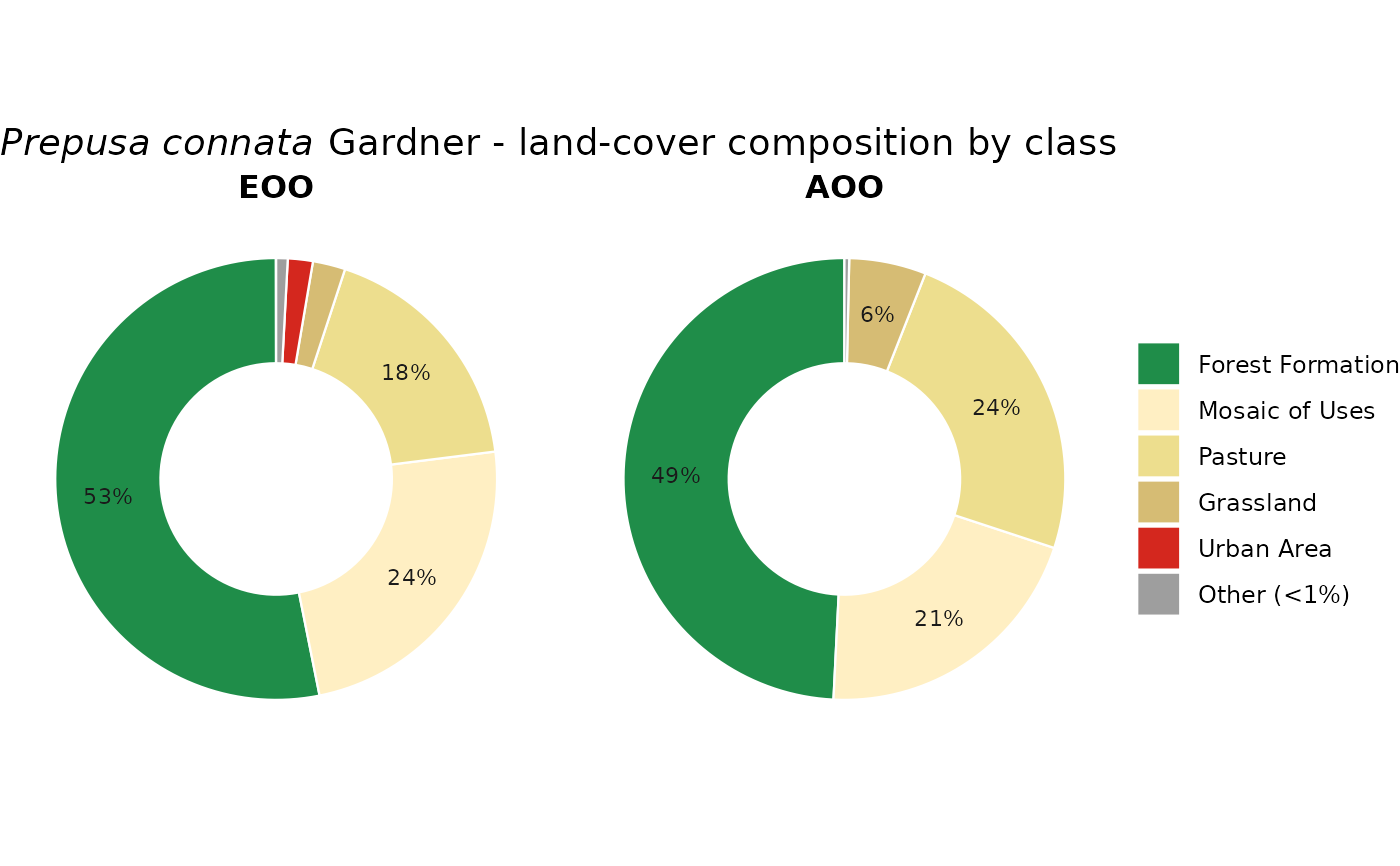
Two side-by-side donut (ring) charts summarising the MapBiomas composition of the Extent of Occurrence (EOO) and Area of Occupancy (AOO) of a species, in the official MapBiomas colours. Slices can be individual land-cover classes (by = "class") or the four conservation groups (by = "group"). Designed to be exported as a transparent-background PNG (all panel/plot/legend backgrounds are transparent), and the interactive plotly version (via mas_plotly) adds outside labels with leader lines and a transparent export.

Usage

plot_conversion_donut(
  assessment,
  species = NULL,
  by = c("class", "group"),
  lang = c("en", "pt")
)

Arguments

assessment

A geoconv_assessment from assess_species (run with mapbiomas = TRUE).

species

Optional species name. NULL (default) uses the first assessed species.

by

"class" (default) for one ring slice per MapBiomas class, or "group" for the Natural / Altered / Water / Other summary.

lang

"en" (default) or "pt" for slice labels.

Value

A ggplot object (with mappingAS metadata attached in attribute "mas" so mas_plotly can build the interactive donut). Stops with an informative message if no class data are available.

Examples

# \donttest{
occ <- read_occurrences(system.file("extdata", "example_occurrences.csv",
                                    package = "mappingAS"))
# reads MapBiomas (one year; the multi-year habitat trend is skipped)
res <- assess_species(occ, year = 2024, infer_decline_from_habitat = FALSE,
                      verbose = FALSE)
plot_conversion_donut(res, by = "class")

# }