Worked example: Prepusa connata • mappingAS

mappingAS ships with a small occurrence table (example_occurrences.csv) for three Brazilian mountain endemics. Here we screen one of them — Prepusa connata Gardner (Gentianaceae), from the Serra dos Órgãos / Serra da Mantiqueira region — against Criterion B of the IUCN Red List.

The range metrics below run offline, from the points alone. The habitat, fire, protected-area and report steps are shown as code because they read MapBiomas / WDPA data over the network.

1. Read the occurrences

library(mappingAS)
library(sf)

occ <- read_occurrences(
  system.file("extdata", "example_occurrences.csv", package = "mappingAS")
)

# keep just Prepusa connata
pc <- occ[grepl("Prepusa connata", occ$species), ]
nrow(pc)
#> [1] 5

2. Extent of Occurrence and Area of Occupancy

Both are computed on a data-centred equal-area projection, so the areas are in honest square kilometres regardless of where on Earth the species lives.

eoo <- calc_eoo(pc)   # minimum convex polygon
aoo <- calc_aoo(pc)   # occupied 2 km grid cells

c(EOO_km2 = round(eoo$area_km2, 1),
  AOO_km2 = round(aoo$area_km2, 1))
#> EOO_km2 AOO_km2 
#>    2468      16

3. Provisional Criterion B category

iucn_criterion_B() turns the two sizes into the provisional category and its IUCN code notation. Called with the sizes alone, as here, the number of locations is unknown and a continuing decline is assumed, so this is a screening result that does not replace a formal assessment.

cat_B <- iucn_criterion_B(eoo_km2 = eoo$area_km2, aoo_km2 = aoo$area_km2)
cat_B$code
#> [1] "NT (meets B size only)"

4. Map the range

library(ggplot2)

hull_wgs <- st_transform(eoo$hull, 4326)   # the EOO polygon, back in lon/lat

ggplot() +
  geom_sf(data = hull_wgs, fill = "#2c6e49", alpha = 0.18, colour = "#2c6e49",
          linewidth = 0.6) +
  geom_sf(data = pc, colour = "#bc4749", size = 2.4) +
  labs(
    title = expression(italic("Prepusa connata") ~ "— EOO and occurrences"),
    subtitle = sprintf("EOO = %s km² · AOO = %s km² · %s",
                       round(eoo$area_km2), round(aoo$area_km2), cat_B$code),
    x = NULL, y = NULL
  ) +
  theme_minimal(base_size = 12)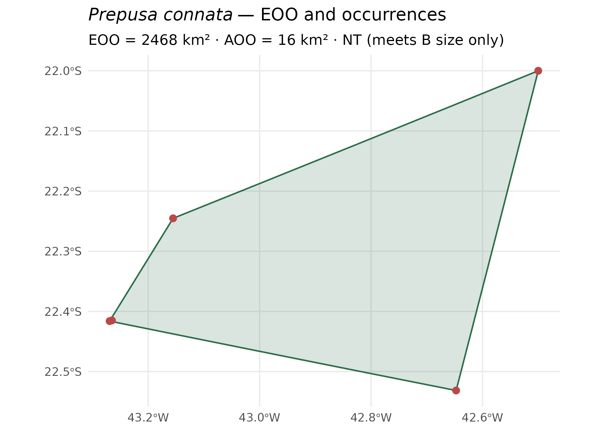

5. Add habitat conversion, fire and protected areas

The one-call pipeline layers MapBiomas land cover, MapBiomas Fire and the global WDPA onto the same range. These read data over the network, so the code is shown rather than run here.

res <- assess_species(
  pc,
  year      = 2024,
  mapbiomas = TRUE,   # % converted vs natural land cover within EOO/AOO
  fire      = TRUE,   # burned-area share and fire time series
  wdpa      = TRUE    # overlap with protected areas (global WDPA)
)

res$summary          # one tidy row: EOO, AOO, category, % converted, % burned…
class_table(res)     # full per-land-cover-class breakdown

# Interactive and publication-ready outputs:
map_species(res)         # Leaflet map (points, EOO, AOO, land cover, fire, PAs)
plot_conversion(res)     # converted vs natural, stacked bar
plot_timeseries(cover_timeseries(res))  # land-cover change over time

6. Write the assessment report

# Self-contained HTML (also "txt" or, with the 'officer' package, "docx"):
assessment_report(res, output = "html", file = "prepusa_connata_assessment.html")

# Export the ranges as spatial data (shapefile / GeoPackage) and the
# clipped land-cover raster as GeoTIFF:
export_ranges(res, dir = "ranges", format = "gpkg")

7. The Shiny application

Everything above — upload, EOO/AOO, habitat conversion, fire, protected areas, maps, charts, report and exports — is wrapped in an interactive Shiny app, the recommended entry point when you don’t want to write code.

run_app()                      # opens in your browser
run_app(max_upload_mb = 2048)  # allow very large occurrence tables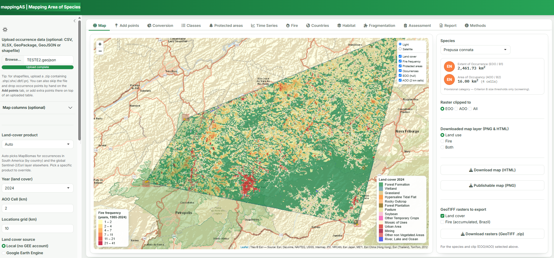

The mappingAS Shiny application

▶ Run it yourself: the app runs locally in your browser — install the package and call run_app() (above). No account or server needed.

Caveats

The category produced is provisional and for screening only. It reflects the EOO/AOO size thresholds of Criterion B with sub-conditions that are estimated (locations, the trend of natural habitat) or assumed, and the assessor must still confirm severe fragmentation, continuing decline and extreme fluctuation for a formal IUCN Red List assessment.